Lab 04: fitting probability distributions to your data using scipy.stats#
CCNY EAS 42000/A42000, Fall 2025, 2025/10/15, Prof. Spencer Hill
SUMMARY: We use xarray to load the netCDF file containing the Central Park weather station daily data from disk, and then a combination of xarray and scipy to fit parametric probability distributions to the data.
Preliminaries#
Import needed python packages#
from matplotlib import pyplot as plt  # for plotting
import numpy as np # for working with arrays of numerical values
import scipy  # for fitting PDFs
import xarray as xr  # for loading data and subsequent analyses
Load the Central Park data into this python session#
Explanation of data downloading logic (if you’re interested)
To make these Jupyter notebooks work when launched to Google Colab—which you can do by clicking the “rocket” icon in the top right from the rendered version of this page on the web—we need some logic that downloads the data.
While we’re at it, we use the file’s “hash” to check that it has not been altered or corrupted from its original version. We do this whether or not you’ve downloaded the file, since it’s possible to (accidentally) modify the netCDF file on disk after you downloaded it.
In the rendered HTML version of the site, this cell is hidden, since otherwise it’s a bit distracting. But you can click on it to reveal its content.
If you’re in a Google Colab session, you don’t need to modify anything in that cell; just run it. Otherwise, modify the LOCAL_DATA_DIR variable defined in the next python cell to point to where the dataset lives on your machine—or where you want it to be downloaded to if you don’t have it already.
import xarray as xr

# `DATA_PATH` variable was created by the hidden cell just above.
# Un-hide that cell if you want to see the details.
ds_cp = xr.open_dataset(DATA_PATH)
ds_cp
<xarray.Dataset> Size: 5MB
Dimensions:        (time: 56520)
Coordinates:
  * time           (time) datetime64[ns] 452kB 1869-01-01 ... 2023-09-30
Data variables:
    temp_max       (time) int64 452kB ...
    temp_min       (time) int64 452kB ...
    temp_avg       (time) float64 452kB ...
    temp_anom      (time) float64 452kB ...
    heat_deg_days  (time) int64 452kB ...
    cool_deg_days  (time) int64 452kB ...
    precip         (time) float64 452kB ...
    snow_fall      (time) float64 452kB ...
snow_depth (time) int64 452kB ...Fit a PDF to the Central Park data using scipy.stats#
There are a ton of available distributions in scipy.stats. You can see a complete list along with other useful information on the associated docs page.
We can also see them, along with everything else defined within scipy.stats, using the built-in dir function:
dir(scipy.stats)
['Binomial',
 'BootstrapMethod',
 'CensoredData',
 'ConstantInputWarning',
 'Covariance',
 'DegenerateDataWarning',
 'FitError',
 'Mixture',
 'MonteCarloMethod',
 'NearConstantInputWarning',
 'Normal',
 'PermutationMethod',
 'Uniform',
 '__all__',
 '__builtins__',
 '__cached__',
 '__doc__',
 '__file__',
 '__loader__',
 '__name__',
 '__package__',
 '__path__',
 '__spec__',
 '_ansari_swilk_statistics',
 '_axis_nan_policy',
 '_biasedurn',
 '_binned_statistic',
 '_binomtest',
 '_bws_test',
 '_censored_data',
 '_common',
 '_constants',
 '_continuous_distns',
 '_correlation',
 '_covariance',
 '_crosstab',
 '_discrete_distns',
 '_distn_infrastructure',
 '_distr_params',
 '_distribution_infrastructure',
 '_entropy',
 '_finite_differences',
 '_fit',
 '_hypotests',
 '_kde',
 '_ksstats',
 '_levy_stable',
 '_mannwhitneyu',
 '_mgc',
 '_morestats',
 '_mstats_basic',
 '_mstats_extras',
 '_multicomp',
 '_multivariate',
 '_new_distributions',
 '_odds_ratio',
 '_page_trend_test',
 '_probability_distribution',
 '_qmc',
 '_qmc_cy',
 '_qmvnt',
 '_qmvnt_cy',
 '_quantile',
 '_rcont',
 '_relative_risk',
 '_resampling',
 '_sensitivity_analysis',
 '_sobol',
 '_stats',
 '_stats_mstats_common',
 '_stats_py',
 '_stats_pythran',
 '_survival',
 '_tukeylambda_stats',
 '_variation',
 '_warnings_errors',
 '_wilcoxon',
 'abs',
 'alexandergovern',
 'alpha',
 'anderson',
 'anderson_ksamp',
 'anglit',
 'ansari',
 'arcsine',
 'argus',
 'barnard_exact',
 'bartlett',
 'bayes_mvs',
 'bernoulli',
 'beta',
 'betabinom',
 'betanbinom',
 'betaprime',
 'biasedurn',
 'binned_statistic',
 'binned_statistic_2d',
 'binned_statistic_dd',
 'binom',
 'binomtest',
 'boltzmann',
 'bootstrap',
 'boschloo_exact',
 'boxcox',
 'boxcox_llf',
 'boxcox_normmax',
 'boxcox_normplot',
 'bradford',
 'brunnermunzel',
 'burr',
 'burr12',
 'bws_test',
 'cauchy',
 'chatterjeexi',
 'chi',
 'chi2',
 'chi2_contingency',
 'chisquare',
 'circmean',
 'circstd',
 'circvar',
 'combine_pvalues',
 'contingency',
 'cosine',
 'cramervonmises',
 'cramervonmises_2samp',
 'crystalball',
 'cumfreq',
 'describe',
 'dgamma',
 'differential_entropy',
 'directional_stats',
 'dirichlet',
 'dirichlet_multinomial',
 'distributions',
 'dlaplace',
 'dpareto_lognorm',
 'dunnett',
 'dweibull',
 'ecdf',
 'energy_distance',
 'entropy',
 'epps_singleton_2samp',
 'erlang',
 'exp',
 'expectile',
 'expon',
 'exponnorm',
 'exponpow',
 'exponweib',
 'f',
 'f_oneway',
 'false_discovery_control',
 'fatiguelife',
 'find_repeats',
 'fisher_exact',
 'fisk',
 'fit',
 'fligner',
 'foldcauchy',
 'foldnorm',
 'friedmanchisquare',
 'gamma',
 'gausshyper',
 'gaussian_kde',
 'genexpon',
 'genextreme',
 'gengamma',
 'genhalflogistic',
 'genhyperbolic',
 'geninvgauss',
 'genlogistic',
 'gennorm',
 'genpareto',
 'geom',
 'gibrat',
 'gmean',
 'gompertz',
 'goodness_of_fit',
 'gstd',
 'gumbel_l',
 'gumbel_r',
 'gzscore',
 'halfcauchy',
 'halfgennorm',
 'halflogistic',
 'halfnorm',
 'hmean',
 'hypergeom',
 'hypsecant',
 'invgamma',
 'invgauss',
 'invweibull',
 'invwishart',
 'iqr',
 'irwinhall',
 'jarque_bera',
 'jf_skew_t',
 'johnsonsb',
 'johnsonsu',
 'kappa3',
 'kappa4',
 'kde',
 'kendalltau',
 'kruskal',
 'ks_1samp',
 'ks_2samp',
 'ksone',
 'kstat',
 'kstatvar',
 'kstest',
 'kstwo',
 'kstwobign',
 'kurtosis',
 'kurtosistest',
 'landau',
 'laplace',
 'laplace_asymmetric',
 'levene',
 'levy',
 'levy_l',
 'levy_stable',
 'linregress',
 'lmoment',
 'log',
 'loggamma',
 'logistic',
 'loglaplace',
 'lognorm',
 'logrank',
 'logser',
 'loguniform',
 'lomax',
 'make_distribution',
 'mannwhitneyu',
 'matrix_normal',
 'maxwell',
 'median_abs_deviation',
 'median_test',
 'mielke',
 'mode',
 'moment',
 'monte_carlo_test',
 'mood',
 'morestats',
 'moyal',
 'mstats',
 'mstats_basic',
 'mstats_extras',
 'multinomial',
 'multiscale_graphcorr',
 'multivariate_hypergeom',
 'multivariate_normal',
 'multivariate_t',
 'mvn',
 'mvsdist',
 'nakagami',
 'nbinom',
 'ncf',
 'nchypergeom_fisher',
 'nchypergeom_wallenius',
 'nct',
 'ncx2',
 'nhypergeom',
 'norm',
 'normal_inverse_gamma',
 'normaltest',
 'norminvgauss',
 'obrientransform',
 'order_statistic',
 'ortho_group',
 'page_trend_test',
 'pareto',
 'pearson3',
 'pearsonr',
 'percentileofscore',
 'permutation_test',
 'planck',
 'pmean',
 'pointbiserialr',
 'poisson',
 'poisson_binom',
 'poisson_means_test',
 'power',
 'power_divergence',
 'powerlaw',
 'powerlognorm',
 'powernorm',
 'ppcc_max',
 'ppcc_plot',
 'probplot',
 'qmc',
 'quantile',
 'quantile_test',
 'randint',
 'random_correlation',
 'random_table',
 'rankdata',
 'ranksums',
 'rayleigh',
 'rdist',
 'recipinvgauss',
 'reciprocal',
 'rel_breitwigner',
 'relfreq',
 'rice',
 'rv_continuous',
 'rv_discrete',
 'rv_histogram',
 'scoreatpercentile',
 'sem',
 'semicircular',
 'shapiro',
 'siegelslopes',
 'sigmaclip',
 'skellam',
 'skew',
 'skewcauchy',
 'skewnorm',
 'skewtest',
 'sobol_indices',
 'somersd',
 'spearmanr',
 'special_ortho_group',
 'stats',
 'studentized_range',
 't',
 'test',
 'theilslopes',
 'tiecorrect',
 'tmax',
 'tmean',
 'tmin',
 'trapezoid',
 'triang',
 'trim1',
 'trim_mean',
 'trimboth',
 'truncate',
 'truncexpon',
 'truncnorm',
 'truncpareto',
 'truncweibull_min',
 'tsem',
 'tstd',
 'ttest_1samp',
 'ttest_ind',
 'ttest_ind_from_stats',
 'ttest_rel',
 'tukey_hsd',
 'tukeylambda',
 'tvar',
 'uniform',
 'uniform_direction',
 'unitary_group',
 'variation',
 'vonmises',
 'vonmises_fisher',
 'vonmises_line',
 'wald',
 'wasserstein_distance',
 'wasserstein_distance_nd',
 'weibull_max',
 'weibull_min',
 'weightedtau',
 'wilcoxon',
 'wishart',
 'wrapcauchy',
 'yeojohnson',
 'yeojohnson_llf',
 'yeojohnson_normmax',
 'yeojohnson_normplot',
 'yulesimon',
 'zipf',
 'zipfian',
 'zmap',
 'zscore']
To start, let’s use the normal function, which is scipy.stats.norm:
help(scipy.stats.norm)
Help on norm_gen in module scipy.stats._continuous_distns:

<scipy.stats._continuous_distns.norm_gen object>
    A normal continuous random variable.

    The location (``loc``) keyword specifies the mean.
    The scale (``scale``) keyword specifies the standard deviation.

    As an instance of the `rv_continuous` class, `norm` object inherits from it
    a collection of generic methods (see below for the full list),
    and completes them with details specific for this particular distribution.

    Methods
    -------
    rvs(loc=0, scale=1, size=1, random_state=None)
        Random variates.
    pdf(x, loc=0, scale=1)
        Probability density function.
    logpdf(x, loc=0, scale=1)
        Log of the probability density function.
    cdf(x, loc=0, scale=1)
        Cumulative distribution function.
    logcdf(x, loc=0, scale=1)
        Log of the cumulative distribution function.
    sf(x, loc=0, scale=1)
        Survival function  (also defined as ``1 - cdf``, but `sf` is sometimes more accurate).
    logsf(x, loc=0, scale=1)
        Log of the survival function.
    ppf(q, loc=0, scale=1)
        Percent point function (inverse of ``cdf`` --- percentiles).
    isf(q, loc=0, scale=1)
        Inverse survival function (inverse of ``sf``).
    moment(order, loc=0, scale=1)
        Non-central moment of the specified order.
    stats(loc=0, scale=1, moments='mv')
        Mean('m'), variance('v'), skew('s'), and/or kurtosis('k').
    entropy(loc=0, scale=1)
        (Differential) entropy of the RV.
    fit(data)
        Parameter estimates for generic data.
        See `scipy.stats.rv_continuous.fit <https://docs.scipy.org/doc/scipy/reference/generated/scipy.stats.rv_continuous.fit.html#scipy.stats.rv_continuous.fit>`__ for detailed documentation of the
        keyword arguments.
    expect(func, args=(), loc=0, scale=1, lb=None, ub=None, conditional=False, **kwds)
        Expected value of a function (of one argument) with respect to the distribution.
    median(loc=0, scale=1)
        Median of the distribution.
    mean(loc=0, scale=1)
        Mean of the distribution.
    var(loc=0, scale=1)
        Variance of the distribution.
    std(loc=0, scale=1)
        Standard deviation of the distribution.
    interval(confidence, loc=0, scale=1)
        Confidence interval with equal areas around the median.

    Notes
    -----
    The probability density function for `norm` is:

    .. math::

        f(x) = \frac{\exp(-x^2/2)}{\sqrt{2\pi}}

    for a real number :math:`x`.

    The probability density above is defined in the "standardized" form. To shift
    and/or scale the distribution use the ``loc`` and ``scale`` parameters.
    Specifically, ``norm.pdf(x, loc, scale)`` is identically
    equivalent to ``norm.pdf(y) / scale`` with
    ``y = (x - loc) / scale``. Note that shifting the location of a distribution
    does not make it a "noncentral" distribution; noncentral generalizations of
    some distributions are available in separate classes.

    Examples
    --------
    >>> import numpy as np
    >>> from scipy.stats import norm
    >>> import matplotlib.pyplot as plt
    >>> fig, ax = plt.subplots(1, 1)

    Get the support:


    >>> lb, ub = norm.support()

    Calculate the first four moments:

    >>> mean, var, skew, kurt = norm.stats(moments='mvsk')

    Display the probability density function (``pdf``):

    >>> x = np.linspace(norm.ppf(0.01),
    ...                 norm.ppf(0.99), 100)
    >>> ax.plot(x, norm.pdf(x),
    ...        'r-', lw=5, alpha=0.6, label='norm pdf')

    Alternatively, the distribution object can be called (as a function)
    to fix the shape, location and scale parameters. This returns a "frozen"
    RV object holding the given parameters fixed.

    Freeze the distribution and display the frozen ``pdf``:

    >>> rv = norm()
    >>> ax.plot(x, rv.pdf(x), 'k-', lw=2, label='frozen pdf')

    Check accuracy of ``cdf`` and ``ppf``:

    >>> vals = norm.ppf([0.001, 0.5, 0.999])
    >>> np.allclose([0.001, 0.5, 0.999], norm.cdf(vals))
    True

    Generate random numbers:

    >>> r = norm.rvs(size=1000)

    And compare the histogram:

    >>> ax.hist(r, density=True, bins='auto', histtype='stepfilled', alpha=0.2)
    >>> ax.set_xlim([x[0], x[-1]])
    >>> ax.legend(loc='best', frameon=False)
    >>> plt.show()
Let’s start with daily minimum temperatures in the month of May:
temp_min_may = ds_cp["temp_min"].where(ds_cp["time"].dt.month == 5, drop=True)
temp_min_may
<xarray.DataArray 'temp_min' (time: 4805)> Size: 38kB
array([42.,  0.,  0., ..., 59., 55., 51.], shape=(4805,))
Coordinates:
  * time     (time) datetime64[ns] 38kB 1869-05-01 1869-05-02 ... 2023-05-31
Attributes:
units: degrees FFirst let’s plot it’s histogram:
temp_min_may.plot.hist(density=True)
# could also use plt.hist(temp_min_may)
(array([0.00021907, 0.        , 0.        , 0.        , 0.00052029,
        0.01377403, 0.05561641, 0.0423079 , 0.01659456, 0.00254669]),
 array([ 0. ,  7.6, 15.2, 22.8, 30.4, 38. , 45.6, 53.2, 60.8, 68.4, 76. ]),
 <BarContainer object of 10 artists>)
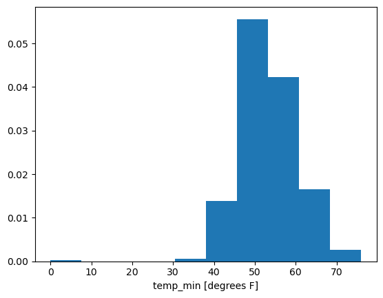
We see here the spurious 0 values. So let’s drop those:
temp_min_may = temp_min_may.where(temp_min_may != 0, drop=True)
Now we can try the histogram again:
temp_min_may.plot.hist(density=True, bins=15)
(array([0.00028427, 0.00106601, 0.00369549, 0.01435556, 0.02949286,
        0.04704645, 0.06346296, 0.06140201, 0.04740179, 0.03176701,
        0.02025414, 0.01179715, 0.00575644, 0.00248735, 0.0006396 ]),
 array([32.        , 34.93333333, 37.86666667, 40.8       , 43.73333333,
        46.66666667, 49.6       , 52.53333333, 55.46666667, 58.4       ,
        61.33333333, 64.26666667, 67.2       , 70.13333333, 73.06666667,
        76.        ]),
 <BarContainer object of 15 artists>)
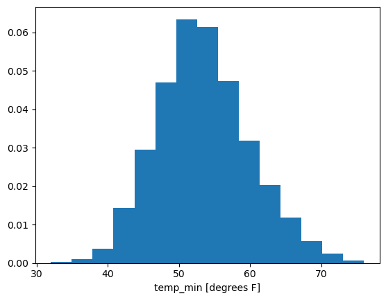
That looks pretty normal—as in, pretty Gaussian—to me!
So let’s proceed with fitting a normal distribution to the data.
To do so we use the .fit method of scipy.stats.norm. You simply give it the data you want to fit as the sole argument, and it returns the best-fit values of both of the normal distribution’s parameters: the mean \(\mu\) and standard deviation \(\sigma\).
mean, stdev = scipy.stats.norm.fit(temp_min_may)
mean, stdev
(np.float64(53.42172190952679), np.float64(6.63132999778397))
This means that the best-fit normal distribution for this data has a mean near 53.4\(^\circ\)F and a standard deviation near 6.6\(^\circ\)F
Now let’s overlay this on the histogram to inspect by eye how well it performs.
First, we’ll create a “frozen” normal PDF by specifying these values of the mean and standard deviation in a new call to scipy.stats.norm.
Note: the mean is called loc, and the standard deviation is called scale, because these are shared names across all distributions…different distributions have different parameters and names for them, and so scipy uses these “universal” names of loc and scale (along with others).
normal_for_tmin_may = scipy.stats.norm(loc=mean, scale=stdev)
normal_for_tmin_may
<scipy.stats._distn_infrastructure.rv_continuous_frozen at 0x7f2d64a9a660>
Now we can call this object’s pdf method, giving it any point or points we want to know the PDF value at:
print(normal_for_tmin_may.pdf(50))  # the value of this PDF at 50 deg F
print(normal_for_tmin_may.pdf([40, 100]))  # the PDF's value at the two points 40 deg F and 100 deg F
0.05266161442811993
[7.75820374e-03 1.16437434e-12]
What we want to do is visually inspect how this PDF compares to our histogram above across the whole range of values.
To do that, we’ll compute the PDF at a whole bunch of individual values spanning that range, and then plot the line connecting all those individual values.
To do so, we’ll create the array of x values over which the values of this distribution’s PDF will be plotted.
To do this we’ll make use of numpy’s linspace function, which creates an array of equally spaced points between two specified endpoints:
help(np.linspace)
Help on _ArrayFunctionDispatcher in module numpy:

linspace(
    start,
    stop,
    num=50,
    endpoint=True,
    retstep=False,
    dtype=None,
    axis=0,
    *,
    device=None
)
    Return evenly spaced numbers over a specified interval.

    Returns `num` evenly spaced samples, calculated over the
    interval [`start`, `stop`].

    The endpoint of the interval can optionally be excluded.

    .. versionchanged:: 1.20.0
        Values are rounded towards ``-inf`` instead of ``0`` when an
        integer ``dtype`` is specified. The old behavior can
        still be obtained with ``np.linspace(start, stop, num).astype(int)``

    Parameters
    ----------
    start : array_like
        The starting value of the sequence.
    stop : array_like
        The end value of the sequence, unless `endpoint` is set to False.
        In that case, the sequence consists of all but the last of ``num + 1``
        evenly spaced samples, so that `stop` is excluded.  Note that the step
        size changes when `endpoint` is False.
    num : int, optional
        Number of samples to generate. Default is 50. Must be non-negative.
    endpoint : bool, optional
        If True, `stop` is the last sample. Otherwise, it is not included.
        Default is True.
    retstep : bool, optional
        If True, return (`samples`, `step`), where `step` is the spacing
        between samples.
    dtype : dtype, optional
        The type of the output array.  If `dtype` is not given, the data type
        is inferred from `start` and `stop`. The inferred dtype will never be
        an integer; `float` is chosen even if the arguments would produce an
        array of integers.
    axis : int, optional
        The axis in the result to store the samples.  Relevant only if start
        or stop are array-like.  By default (0), the samples will be along a
        new axis inserted at the beginning. Use -1 to get an axis at the end.
    device : str, optional
        The device on which to place the created array. Default: None.
        For Array-API interoperability only, so must be ``"cpu"`` if passed.

        .. versionadded:: 2.0.0

    Returns
    -------
    samples : ndarray
        There are `num` equally spaced samples in the closed interval
        ``[start, stop]`` or the half-open interval ``[start, stop)``
        (depending on whether `endpoint` is True or False).
    step : float, optional
        Only returned if `retstep` is True

        Size of spacing between samples.


    See Also
    --------
    arange : Similar to `linspace`, but uses a step size (instead of the
             number of samples).
    geomspace : Similar to `linspace`, but with numbers spaced evenly on a log
                scale (a geometric progression).
    logspace : Similar to `geomspace`, but with the end points specified as
               logarithms.
    :ref:`how-to-partition`

    Examples
    --------
    >>> import numpy as np
    >>> np.linspace(2.0, 3.0, num=5)
    array([2.  , 2.25, 2.5 , 2.75, 3.  ])
    >>> np.linspace(2.0, 3.0, num=5, endpoint=False)
    array([2. ,  2.2,  2.4,  2.6,  2.8])
    >>> np.linspace(2.0, 3.0, num=5, retstep=True)
    (array([2.  ,  2.25,  2.5 ,  2.75,  3.  ]), 0.25)

    Graphical illustration:

    >>> import matplotlib.pyplot as plt
    >>> N = 8
    >>> y = np.zeros(N)
    >>> x1 = np.linspace(0, 10, N, endpoint=True)
    >>> x2 = np.linspace(0, 10, N, endpoint=False)
    >>> plt.plot(x1, y, 'o')
    [<matplotlib.lines.Line2D object at 0x...>]
    >>> plt.plot(x2, y + 0.5, 'o')
    [<matplotlib.lines.Line2D object at 0x...>]
    >>> plt.ylim([-0.5, 1])
    (-0.5, 1)
    >>> plt.show()
xvals_for_norm_fit = np.linspace(temp_min_may.min().values, temp_min_may.max().values, 100)
xvals_for_norm_fit
array([32.        , 32.44444444, 32.88888889, 33.33333333, 33.77777778,
       34.22222222, 34.66666667, 35.11111111, 35.55555556, 36.        ,
       36.44444444, 36.88888889, 37.33333333, 37.77777778, 38.22222222,
       38.66666667, 39.11111111, 39.55555556, 40.        , 40.44444444,
       40.88888889, 41.33333333, 41.77777778, 42.22222222, 42.66666667,
       43.11111111, 43.55555556, 44.        , 44.44444444, 44.88888889,
       45.33333333, 45.77777778, 46.22222222, 46.66666667, 47.11111111,
       47.55555556, 48.        , 48.44444444, 48.88888889, 49.33333333,
       49.77777778, 50.22222222, 50.66666667, 51.11111111, 51.55555556,
       52.        , 52.44444444, 52.88888889, 53.33333333, 53.77777778,
       54.22222222, 54.66666667, 55.11111111, 55.55555556, 56.        ,
       56.44444444, 56.88888889, 57.33333333, 57.77777778, 58.22222222,
       58.66666667, 59.11111111, 59.55555556, 60.        , 60.44444444,
       60.88888889, 61.33333333, 61.77777778, 62.22222222, 62.66666667,
       63.11111111, 63.55555556, 64.        , 64.44444444, 64.88888889,
       65.33333333, 65.77777778, 66.22222222, 66.66666667, 67.11111111,
       67.55555556, 68.        , 68.44444444, 68.88888889, 69.33333333,
       69.77777778, 70.22222222, 70.66666667, 71.11111111, 71.55555556,
       72.        , 72.44444444, 72.88888889, 73.33333333, 73.77777778,
       74.22222222, 74.66666667, 75.11111111, 75.55555556, 76.        ])
fig, ax = plt.subplots()

temp_min_may.plot.hist(ax=ax, density=True, bins=15)

plt.plot(xvals_for_norm_fit, normal_for_tmin_may.pdf(xvals_for_norm_fit))
[<matplotlib.lines.Line2D at 0x7f2d6477ca50>]
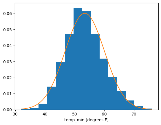
Nice! By visual inspection, this sample of daily minimum temperatures in the month of May for 1869-2023 looks pretty well approximated by a normal distribution!