Lab 03: computing empirical probabilities, empirical CDFs, and empirical PDFs#
CCNY EAS 42000/A42000, Fall 2025, 2025/10/08, Prof. Spencer Hill
SUMMARY: We use xarray to load the netCDF file containing the Central Park weather station daily data from disk, and then a combination of xarray and scipy to compute empirical probabilites, CDFs, and PDFs from that data.
Preliminaries#
Notebook magic commands#
(There are two of these. The first you should include; the second only matters if you are on a Mac computer with a Retina display.)
# Turn on rendering of matplotlib figures directly in the notebook.
%matplotlib inline
# OPTIONAL.  Make figures higher resolution on my Macbook.
%config InlineBackend.figure_format = "retina"
Imports#
from matplotlib import pyplot as plt  # for plotting
import scipy  # for computing empirical CDFs
import xarray as xr  # for loading data and subsequent analyses
Check that your version of scipy has the scipy.stats.ecdf function, which was introduced in 2023#
scipy.stats.ecdf
<function scipy.stats._survival.ecdf(sample: 'npt.ArrayLike | CensoredData') -> scipy.stats._survival.ECDFResult>
If the cell just above gives you a NameError, that means that you don’t have a recent enough version of scipy. You can resolve this by updating your installed scipy to a newer version using pip or conda. Consult HW03 for further instructions.
Load the Central Park data into this python session#
Explanation of data downloading logic (if you’re interested)
To make these Jupyter notebooks work when launched to Google Colab—which you can do by clicking the “rocket” icon in the top right from the rendered version of this page on the web—we need some logic that downloads the data.
While we’re at it, we use the file’s “hash” to check that it has not been altered or corrupted from its original version. We do this whether or not you’ve downloaded the file, since it’s possible to (accidentally) modify the netCDF file on disk after you downloaded it.
In the rendered HTML version of the site, this cell is hidden, since otherwise it’s a bit distracting. But you can click on it to reveal its content.
If you’re in a Google Colab session, you don’t need to modify anything in that cell; just run it. Otherwise, modify the LOCAL_DATA_DIR variable defined in the next python cell to point to where the dataset lives on your machine—or where you want it to be downloaded to if you don’t have it already.
import xarray as xr

# `DATA_PATH` variable was created by the hidden cell just above.
# Un-hide that cell if you want to see the details.
ds_cp = xr.open_dataset(DATA_PATH)
ds_cp
<xarray.Dataset> Size: 5MB
Dimensions:        (time: 56520)
Coordinates:
  * time           (time) datetime64[ns] 452kB 1869-01-01 ... 2023-09-30
Data variables:
    temp_max       (time) int64 452kB ...
    temp_min       (time) int64 452kB ...
    temp_avg       (time) float64 452kB ...
    temp_anom      (time) float64 452kB ...
    heat_deg_days  (time) int64 452kB ...
    cool_deg_days  (time) int64 452kB ...
    precip         (time) float64 452kB ...
    snow_fall      (time) float64 452kB ...
snow_depth (time) int64 452kB ...Empirical probabilities#
Recall: the empirical probability of an event \(E\) is simply the number of times \(E\) occurs, divided by the total number of times it could have occurred.
The built-in len function is helpful for this.
Technical aside: jupyter question mark ? vs. built-in help function#
Recall that in a Jupyter session, entering the name of an object followed by a question mark will display information about that object.
If you’re reading this as the rendered HTML of this notebook, cells that call Jupyter’s ? feature will not actually show anything, for technical reasons. For example:
len?
But if you run this yourself in a jupyter session, you will get output, specifically:
Signature: len(obj, /)
Docstring: Return the number of items in a container.
Type:      builtin_function_or_method
As such, I’ll use the builtin help function, which gives you similar output and does render in both a running notebook and the rendered HTML.
help(len)
Help on built-in function len in module builtins:

len(obj, /)
    Return the number of items in a container.
The downsides of help compared to ? are:
helpis not as detailed,not formatted as nicely (including colors)
requires typing more characters.
Example: days with average temperature > 70F#
The numerator is simply the number of days meeting this condition.
How do we do this in python/xarray? The first tsep is really simple. Simply use the “greater than” operator, >, directly on the xr.DataArray object:
ds_cp["temp_avg"] > 70 # this MASKS out values not meeting this condition
<xarray.DataArray 'temp_avg' (time: 56520)> Size: 57kB
array([False, False, False, ..., False, False, False], shape=(56520,))
Coordinates:
  * time     (time) datetime64[ns] 452kB 1869-01-01 1869-01-02 ... 2023-09-30
The resulting xr.DataArray is identical in shape to the original ds_cp["temp_avg"], but its values are all bool: they are True where the condition is satisfied and False where it is not satisfied.
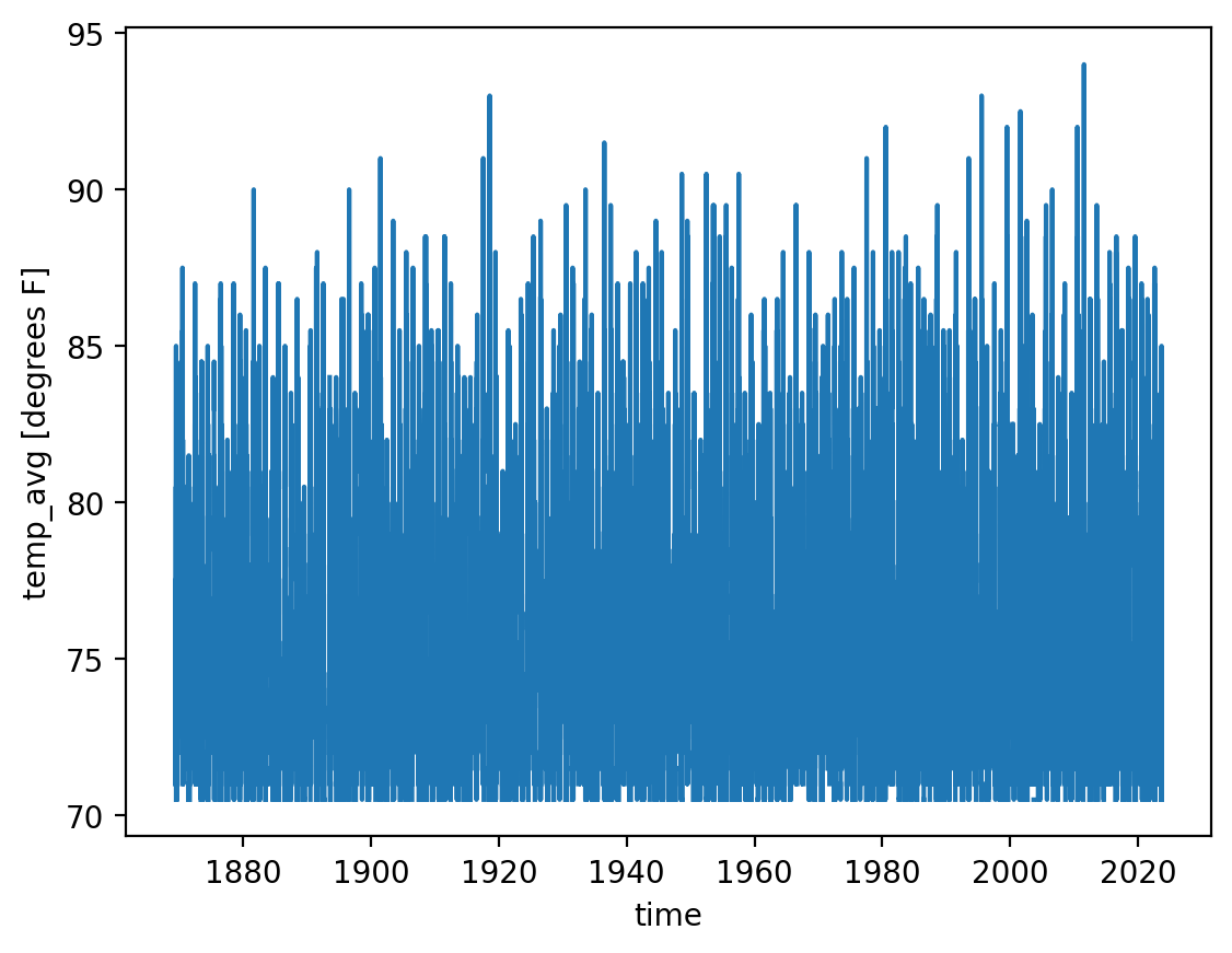
As a sanity check, let’s plot this new array. You’ll see that all of its values are 70F or greater, as intended:
ds_cp["temp_avg"].where(ds_cp["temp_avg"] > 70).plot()
[<matplotlib.lines.Line2D at 0x7f61b1f0afd0>]
Now let’s assign this result to its own variable for use later on:
is_temp_avg_above_70 = ds_cp["temp_avg"] > 70
Next, we use is_temp_avg_above_70 as the input to the where method of xr.DataArray to create a mask that restricts to only the data points meeting that condition.
We also use set drop=True, so that the points not meeting this condition are dropped entirely. (The default, drop=False, leaves them in place but replaces their values with np.nan, which means “Not a Number.”)
temp_avg_above_70 = ds_cp["temp_avg"].where(is_temp_avg_above_70, drop=True)
temp_avg_above_70
<xarray.DataArray 'temp_avg' (time: 13401)> Size: 107kB
array([71.5, 71.5, 74.5, ..., 75.5, 75. , 74.5], shape=(13401,))
Coordinates:
  * time     (time) datetime64[ns] 107kB 1869-05-12 1869-05-25 ... 2023-09-13
Attributes:
units: degrees FFrom visually inspecting this output, you can see that the there are 13,401 days satisfying this condition.
You could, if you wanted, then hardcode that value into a new variable. E.g. num_days_above70 = 13401.
However, we want to avoid hardcoding numerical values in like this whenever possible. Instead, we want to write code that outputs that 13401 value directly.
As noted above, a really easy way of doing that is with len:
len(temp_avg_above_70)
13401
So let’s store that in its own variable:
num_days_temp_avg_above_70 = len(temp_avg_above_70)
num_days_temp_avg_above_70
13401
Alternative approach: use the count method
As is often the case in programming, there are multiple ways of accomplishing the same thing here. One equally elegant solution would be to use the builtin count method of xr.DataArray: ds_cp["temp_avg"].where(is_temp_avg_above_70).count().
Notice there you don’t have to set drop=True: count automatically ignores masked values, meaning values that are nan.
(Hat tip to Storm H. for showing me count!)
Now we have the numerator. The denominator is much easier. It’s simply the total number of days in the dataset:
total_days = len(ds_cp["temp_avg"])
total_days
56520
Finally, we can put it all together:
# Q1: P(temp_avg > 70F)
denom = total_days
numer = num_days_temp_avg_above_70
emp_prob = numer / denom
print(f"Numerator: {numer}, denominator: {denom}, empirical probability: {emp_prob}")
Numerator: 13401, denominator: 56520, empirical probability: 0.23710191082802548
Selecting individual months of the year#
Often, including for some of the empirical probability problems on this assignment, you need to select a subset in time of your dataset.
For example, one of the problems asks you about days in the month of July.
In this case and often, the time coordinate is stored as a special type of object, which you can think of as a kind of calendar.
These calendar objects have lots of handy builtin tools for slicing and dicing time in different ways: by year, by day of the week, by month, etc. etc.
We access these via a special dt accessor, which you get to simply by appending .dt to the time array itself: ds_cp["time"] is the time array, so it’s ds_cp["time"].dt.
Let’s use the builtin dir function to see what all is available to us from this dt accessor:
dir(ds_cp["time"].dt)
['__annotations__',
 '__class__',
 '__class_getitem__',
 '__delattr__',
 '__dict__',
 '__dir__',
 '__doc__',
 '__eq__',
 '__firstlineno__',
 '__format__',
 '__ge__',
 '__getattribute__',
 '__getstate__',
 '__gt__',
 '__hash__',
 '__init__',
 '__init_subclass__',
 '__le__',
 '__lt__',
 '__module__',
 '__ne__',
 '__new__',
 '__orig_bases__',
 '__orig_class__',
 '__parameters__',
 '__reduce__',
 '__reduce_ex__',
 '__repr__',
 '__setattr__',
 '__sizeof__',
 '__slots__',
 '__static_attributes__',
 '__str__',
 '__subclasshook__',
 '__weakref__',
 '_date_field',
 '_obj',
 '_tslib_round_accessor',
 'calendar',
 'ceil',
 'date',
 'day',
 'dayofweek',
 'dayofyear',
 'days_in_month',
 'days_in_year',
 'daysinmonth',
 'decimal_year',
 'floor',
 'hour',
 'is_leap_year',
 'is_month_end',
 'is_month_start',
 'is_quarter_end',
 'is_quarter_start',
 'is_year_end',
 'is_year_start',
 'isocalendar',
 'microsecond',
 'minute',
 'month',
 'nanosecond',
 'quarter',
 'round',
 'season',
 'second',
 'strftime',
 'time',
 'week',
 'weekday',
 'weekofyear',
 'year']
We can access any of these by simply adding them on to the dt. For example, if we want the month:
ds_cp["time"].dt.month
<xarray.DataArray 'month' (time: 56520)> Size: 452kB
array([1, 1, 1, ..., 9, 9, 9], shape=(56520,))
Coordinates:
  * time     (time) datetime64[ns] 452kB 1869-01-01 1869-01-02 ... 2023-09-30
This is an xr.DataArray that is identical to our original time array, but instead of its values being the actual date, the values are the number of the calendar month of that particular date. So the first one, which is January 1, 1869, is 1. Any dates that are in February are 2, and so on through 12 for dates in December.
So putting that all together:
# select just July days
ds_cp.where(ds_cp["time"].dt.month == 7, drop=True)
<xarray.Dataset> Size: 384kB
Dimensions:        (time: 4805)
Coordinates:
  * time           (time) datetime64[ns] 38kB 1869-07-01 ... 2023-07-31
Data variables:
    temp_max       (time) float64 38kB 70.0 76.0 84.0 83.0 ... 89.0 80.0 85.0
    temp_min       (time) float64 38kB 62.0 64.0 70.0 72.0 ... 70.0 66.0 66.0
    temp_avg       (time) float64 38kB 66.0 70.0 77.0 77.5 ... 79.5 73.0 75.5
    temp_anom      (time) float64 38kB -10.3 -6.4 0.4 0.7 ... 5.8 1.9 -4.6 -2.0
    heat_deg_days  (time) float64 38kB 0.0 0.0 0.0 0.0 0.0 ... 0.0 0.0 0.0 0.0
    cool_deg_days  (time) float64 38kB 1.0 5.0 12.0 13.0 ... 19.0 15.0 8.0 11.0
    precip         (time) float64 38kB 0.0 0.0 0.42 0.0 0.0 ... 0.0 0.06 0.0 0.0
    snow_fall      (time) float64 38kB 0.0 0.0 0.0 0.0 0.0 ... 0.0 0.0 0.0 0.0
snow_depth (time) float64 38kB 0.0 0.0 0.0 0.0 0.0 ... 0.0 0.0 0.0 0.0Hint: for another one of the problems, try dt.dayofweek.
Empirical CDFs#
Let’s start by getting some info about the scipy.stats.ecdf function we’ll be using:
# c.f. note above: you can alternatively use `scipy.stats.ecdf?`
help(scipy.stats.ecdf)
Help on function ecdf in module scipy.stats._survival:

ecdf(sample: 'npt.ArrayLike | CensoredData') -> scipy.stats._survival.ECDFResult
    Empirical cumulative distribution function of a sample.

    The empirical cumulative distribution function (ECDF) is a step function
    estimate of the CDF of the distribution underlying a sample. This function
    returns objects representing both the empirical distribution function and
    its complement, the empirical survival function.

    Parameters
    ----------
    sample : 1D array_like or `scipy.stats.CensoredData`
        Besides array_like, instances of `scipy.stats.CensoredData` containing
        uncensored and right-censored observations are supported. Currently,
        other instances of `scipy.stats.CensoredData` will result in a
        ``NotImplementedError``.

    Returns
    -------
    res : `~scipy.stats._result_classes.ECDFResult`
        An object with the following attributes.

        cdf : `~scipy.stats._result_classes.EmpiricalDistributionFunction`
            An object representing the empirical cumulative distribution
            function.
        sf : `~scipy.stats._result_classes.EmpiricalDistributionFunction`
            An object representing the empirical survival function.

        The `cdf` and `sf` attributes themselves have the following attributes.

        quantiles : ndarray
            The unique values in the sample that defines the empirical CDF/SF.
        probabilities : ndarray
            The point estimates of the probabilities corresponding with
            `quantiles`.

        And the following methods:

        evaluate(x) :
            Evaluate the CDF/SF at the argument.

        plot(ax) :
            Plot the CDF/SF on the provided axes.

        confidence_interval(confidence_level=0.95) :
            Compute the confidence interval around the CDF/SF at the values in
            `quantiles`.

    Notes
    -----
    When each observation of the sample is a precise measurement, the ECDF
    steps up by ``1/len(sample)`` at each of the observations [1]_.

    When observations are lower bounds, upper bounds, or both upper and lower
    bounds, the data is said to be "censored", and `sample` may be provided as
    an instance of `scipy.stats.CensoredData`.

    For right-censored data, the ECDF is given by the Kaplan-Meier estimator
    [2]_; other forms of censoring are not supported at this time.

    Confidence intervals are computed according to the Greenwood formula or the
    more recent "Exponential Greenwood" formula as described in [4]_.

    References
    ----------
    .. [1] Conover, William Jay. Practical nonparametric statistics. Vol. 350.
           John Wiley & Sons, 1999.

    .. [2] Kaplan, Edward L., and Paul Meier. "Nonparametric estimation from
           incomplete observations." Journal of the American statistical
           association 53.282 (1958): 457-481.

    .. [3] Goel, Manish Kumar, Pardeep Khanna, and Jugal Kishore.
           "Understanding survival analysis: Kaplan-Meier estimate."
           International journal of Ayurveda research 1.4 (2010): 274.

    .. [4] Sawyer, Stanley. "The Greenwood and Exponential Greenwood Confidence
           Intervals in Survival Analysis."
           https://www.math.wustl.edu/~sawyer/handouts/greenwood.pdf

    Examples
    --------
    **Uncensored Data**

    As in the example from [1]_ page 79, five boys were selected at random from
    those in a single high school. Their one-mile run times were recorded as
    follows.

    >>> sample = [6.23, 5.58, 7.06, 6.42, 5.20]  # one-mile run times (minutes)

    The empirical distribution function, which approximates the distribution
    function of one-mile run times of the population from which the boys were
    sampled, is calculated as follows.

    >>> from scipy import stats
    >>> res = stats.ecdf(sample)
    >>> res.cdf.quantiles
    array([5.2 , 5.58, 6.23, 6.42, 7.06])
    >>> res.cdf.probabilities
    array([0.2, 0.4, 0.6, 0.8, 1. ])

    To plot the result as a step function:

    >>> import matplotlib.pyplot as plt
    >>> ax = plt.subplot()
    >>> res.cdf.plot(ax)
    >>> ax.set_xlabel('One-Mile Run Time (minutes)')
    >>> ax.set_ylabel('Empirical CDF')
    >>> plt.show()

    **Right-censored Data**

    As in the example from [1]_ page 91, the lives of ten car fanbelts were
    tested. Five tests concluded because the fanbelt being tested broke, but
    the remaining tests concluded for other reasons (e.g. the study ran out of
    funding, but the fanbelt was still functional). The mileage driven
    with the fanbelts were recorded as follows.

    >>> broken = [77, 47, 81, 56, 80]  # in thousands of miles driven
    >>> unbroken = [62, 60, 43, 71, 37]

    Precise survival times of the fanbelts that were still functional at the
    end of the tests are unknown, but they are known to exceed the values
    recorded in ``unbroken``. Therefore, these observations are said to be
    "right-censored", and the data is represented using
    `scipy.stats.CensoredData`.

    >>> sample = stats.CensoredData(uncensored=broken, right=unbroken)

    The empirical survival function is calculated as follows.

    >>> res = stats.ecdf(sample)
    >>> res.sf.quantiles
    array([37., 43., 47., 56., 60., 62., 71., 77., 80., 81.])
    >>> res.sf.probabilities
    array([1.   , 1.   , 0.875, 0.75 , 0.75 , 0.75 , 0.75 , 0.5  , 0.25 , 0.   ])

    To plot the result as a step function:

    >>> ax = plt.subplot()
    >>> res.sf.plot(ax)
    >>> ax.set_xlabel('Fanbelt Survival Time (thousands of miles)')
    >>> ax.set_ylabel('Empirical SF')
    >>> plt.show()
OK, so let’s call it on our daily maximum temperature variable:
ecdf_temp_max = scipy.stats.ecdf(ds_cp["temp_max"])
ecdf_temp_max
ECDFResult(cdf=EmpiricalDistributionFunction(quantiles=array([  0.,   2.,   4.,   6.,   7.,   8.,   9.,  10.,  11.,  12.,  13.,
        14.,  15.,  16.,  17.,  18.,  19.,  20.,  21.,  22.,  23.,  24.,
        25.,  26.,  27.,  28.,  29.,  30.,  31.,  32.,  33.,  34.,  35.,
        36.,  37.,  38.,  39.,  40.,  41.,  42.,  43.,  44.,  45.,  46.,
        47.,  48.,  49.,  50.,  51.,  52.,  53.,  54.,  55.,  56.,  57.,
        58.,  59.,  60.,  61.,  62.,  63.,  64.,  65.,  66.,  67.,  68.,
        69.,  70.,  71.,  72.,  73.,  74.,  75.,  76.,  77.,  78.,  79.,
        80.,  81.,  82.,  83.,  84.,  85.,  86.,  87.,  88.,  89.,  90.,
        91.,  92.,  93.,  94.,  95.,  96.,  97.,  98.,  99., 100., 101.,
       102., 103., 104., 106.]), probabilities=array([0.00125619, 0.00127389, 0.00130927, 0.00134466, 0.00143312,
       0.00155697, 0.00166313, 0.00189314, 0.00205237, 0.00228238,
       0.00258316, 0.00290163, 0.00334395, 0.00389243, 0.00442321,
       0.00530786, 0.00631635, 0.00805025, 0.00980184, 0.01224345,
       0.01433121, 0.0170913 , 0.02031139, 0.02430998, 0.02837933,
       0.03324487, 0.03864119, 0.04543524, 0.05276008, 0.06165959,
       0.07050602, 0.08149328, 0.09258669, 0.10546709, 0.11857749,
       0.1329264 , 0.1467799 , 0.16383581, 0.1794586 , 0.19511677,
       0.21081033, 0.22662774, 0.24189667, 0.25711253, 0.2730184 ,
       0.28816348, 0.30380396, 0.32061217, 0.33582803, 0.35053079,
       0.3653574 , 0.38110403, 0.39587757, 0.41070418, 0.42464614,
       0.43973815, 0.45368011, 0.47013447, 0.48533263, 0.50058386,
       0.51516277, 0.53053786, 0.54501062, 0.56008493, 0.57501769,
       0.59117127, 0.6059448 , 0.62344303, 0.63956122, 0.65705945,
       0.67323071, 0.69143666, 0.70872258, 0.72774239, 0.74488677,
       0.76472045, 0.78264331, 0.80493631, 0.82498231, 0.84495754,
       0.864862  , 0.8844126 , 0.90205237, 0.91884289, 0.93382873,
       0.94663836, 0.95787332, 0.96799363, 0.9757431 , 0.98198868,
       0.98733192, 0.99136589, 0.99400212, 0.99600142, 0.99738146,
       0.99837226, 0.99893843, 0.99945152, 0.99966384, 0.99985846,
       0.99992923, 0.99998231, 1.        ])), sf=EmpiricalDistributionFunction(quantiles=array([  0.,   2.,   4.,   6.,   7.,   8.,   9.,  10.,  11.,  12.,  13.,
        14.,  15.,  16.,  17.,  18.,  19.,  20.,  21.,  22.,  23.,  24.,
        25.,  26.,  27.,  28.,  29.,  30.,  31.,  32.,  33.,  34.,  35.,
        36.,  37.,  38.,  39.,  40.,  41.,  42.,  43.,  44.,  45.,  46.,
        47.,  48.,  49.,  50.,  51.,  52.,  53.,  54.,  55.,  56.,  57.,
        58.,  59.,  60.,  61.,  62.,  63.,  64.,  65.,  66.,  67.,  68.,
        69.,  70.,  71.,  72.,  73.,  74.,  75.,  76.,  77.,  78.,  79.,
        80.,  81.,  82.,  83.,  84.,  85.,  86.,  87.,  88.,  89.,  90.,
        91.,  92.,  93.,  94.,  95.,  96.,  97.,  98.,  99., 100., 101.,
       102., 103., 104., 106.]), probabilities=array([9.98743808e-01, 9.98726115e-01, 9.98690729e-01, 9.98655343e-01,
       9.98566879e-01, 9.98443029e-01, 9.98336872e-01, 9.98106865e-01,
       9.97947629e-01, 9.97717622e-01, 9.97416844e-01, 9.97098372e-01,
       9.96656051e-01, 9.96107573e-01, 9.95576787e-01, 9.94692144e-01,
       9.93683652e-01, 9.91949752e-01, 9.90198160e-01, 9.87756546e-01,
       9.85668790e-01, 9.82908705e-01, 9.79688606e-01, 9.75690021e-01,
       9.71620665e-01, 9.66755131e-01, 9.61358811e-01, 9.54564756e-01,
       9.47239915e-01, 9.38340410e-01, 9.29493984e-01, 9.18506723e-01,
       9.07413305e-01, 8.94532909e-01, 8.81422505e-01, 8.67073602e-01,
       8.53220099e-01, 8.36164190e-01, 8.20541401e-01, 8.04883227e-01,
       7.89189667e-01, 7.73372258e-01, 7.58103326e-01, 7.42887473e-01,
       7.26981599e-01, 7.11836518e-01, 6.96196037e-01, 6.79387827e-01,
       6.64171975e-01, 6.49469214e-01, 6.34642604e-01, 6.18895966e-01,
       6.04122435e-01, 5.89295824e-01, 5.75353857e-01, 5.60261854e-01,
       5.46319887e-01, 5.29865534e-01, 5.14667374e-01, 4.99416136e-01,
       4.84837226e-01, 4.69462137e-01, 4.54989384e-01, 4.39915074e-01,
       4.24982307e-01, 4.08828733e-01, 3.94055202e-01, 3.76556971e-01,
       3.60438783e-01, 3.42940552e-01, 3.26769285e-01, 3.08563340e-01,
       2.91277424e-01, 2.72257608e-01, 2.55113234e-01, 2.35279547e-01,
       2.17356688e-01, 1.95063694e-01, 1.75017693e-01, 1.55042463e-01,
       1.35138004e-01, 1.15587403e-01, 9.79476292e-02, 8.11571125e-02,
       6.61712668e-02, 5.33616419e-02, 4.21266808e-02, 3.20063694e-02,
       2.42569002e-02, 1.80113234e-02, 1.26680821e-02, 8.63411182e-03,
       5.99787686e-03, 3.99858457e-03, 2.61854211e-03, 1.62774239e-03,
       1.06157113e-03, 5.48478415e-04, 3.36164190e-04, 1.41542817e-04,
       7.07714084e-05, 1.76928521e-05, 0.00000000e+00])))
Rather than a simple numpy array or xr.DataArray, this creates a ECDFResult object.
From the output, it looks like this has two attributes, cdf and sf. Most likely of course cdf is the one we’re after.
But since we’re not familiar, let’s use help (or the question mark) again to see what we can do with this:
help(ecdf_temp_max)
Help on ECDFResult in module scipy.stats._survival object:

class ECDFResult(builtins.object)
 |  ECDFResult(q, cdf, sf, n, d)
 |
 |  Result object returned by `scipy.stats.ecdf`
 |
 |  Attributes
 |  ----------
 |  cdf : `~scipy.stats._result_classes.EmpiricalDistributionFunction`
 |      An object representing the empirical cumulative distribution function.
 |  sf : `~scipy.stats._result_classes.EmpiricalDistributionFunction`
 |      An object representing the complement of the empirical cumulative
 |      distribution function.
 |
 |  Methods defined here:
 |
 |  __eq__(self, other)
 |      Return self==value.
 |
 |  __init__(self, q, cdf, sf, n, d)
 |      Initialize self.  See help(type(self)) for accurate signature.
 |
 |  __replace__ = _replace(self, /, **changes) from dataclasses
 |
 |  __repr__(self)
 |      Return repr(self).
 |
 |  ----------------------------------------------------------------------
 |  Data descriptors defined here:
 |
 |  __dict__
 |      dictionary for instance variables
 |
 |  __weakref__
 |      list of weak references to the object
 |
 |  ----------------------------------------------------------------------
 |  Data and other attributes defined here:
 |
 |  __annotations__ = {'cdf': <class 'scipy.stats._survival.EmpiricalDistr...
 |
 |  __dataclass_fields__ = {'cdf': Field(name='cdf',type=<class 'scipy.sta...
 |
 |  __dataclass_params__ = _DataclassParams(init=True,repr=True,eq=True,or...
 |
 |  __hash__ = None
 |
 |  __match_args__ = ('cdf', 'sf')
OK, so indeed under the “Attributes” heading, it clearly says that the cdf is what represents the CDF we’re interested in. So let’s take a look:
ecdf_temp_max.cdf
EmpiricalDistributionFunction(quantiles=array([  0.,   2.,   4.,   6.,   7.,   8.,   9.,  10.,  11.,  12.,  13.,
        14.,  15.,  16.,  17.,  18.,  19.,  20.,  21.,  22.,  23.,  24.,
        25.,  26.,  27.,  28.,  29.,  30.,  31.,  32.,  33.,  34.,  35.,
        36.,  37.,  38.,  39.,  40.,  41.,  42.,  43.,  44.,  45.,  46.,
        47.,  48.,  49.,  50.,  51.,  52.,  53.,  54.,  55.,  56.,  57.,
        58.,  59.,  60.,  61.,  62.,  63.,  64.,  65.,  66.,  67.,  68.,
        69.,  70.,  71.,  72.,  73.,  74.,  75.,  76.,  77.,  78.,  79.,
        80.,  81.,  82.,  83.,  84.,  85.,  86.,  87.,  88.,  89.,  90.,
        91.,  92.,  93.,  94.,  95.,  96.,  97.,  98.,  99., 100., 101.,
       102., 103., 104., 106.]), probabilities=array([0.00125619, 0.00127389, 0.00130927, 0.00134466, 0.00143312,
       0.00155697, 0.00166313, 0.00189314, 0.00205237, 0.00228238,
       0.00258316, 0.00290163, 0.00334395, 0.00389243, 0.00442321,
       0.00530786, 0.00631635, 0.00805025, 0.00980184, 0.01224345,
       0.01433121, 0.0170913 , 0.02031139, 0.02430998, 0.02837933,
       0.03324487, 0.03864119, 0.04543524, 0.05276008, 0.06165959,
       0.07050602, 0.08149328, 0.09258669, 0.10546709, 0.11857749,
       0.1329264 , 0.1467799 , 0.16383581, 0.1794586 , 0.19511677,
       0.21081033, 0.22662774, 0.24189667, 0.25711253, 0.2730184 ,
       0.28816348, 0.30380396, 0.32061217, 0.33582803, 0.35053079,
       0.3653574 , 0.38110403, 0.39587757, 0.41070418, 0.42464614,
       0.43973815, 0.45368011, 0.47013447, 0.48533263, 0.50058386,
       0.51516277, 0.53053786, 0.54501062, 0.56008493, 0.57501769,
       0.59117127, 0.6059448 , 0.62344303, 0.63956122, 0.65705945,
       0.67323071, 0.69143666, 0.70872258, 0.72774239, 0.74488677,
       0.76472045, 0.78264331, 0.80493631, 0.82498231, 0.84495754,
       0.864862  , 0.8844126 , 0.90205237, 0.91884289, 0.93382873,
       0.94663836, 0.95787332, 0.96799363, 0.9757431 , 0.98198868,
       0.98733192, 0.99136589, 0.99400212, 0.99600142, 0.99738146,
       0.99837226, 0.99893843, 0.99945152, 0.99966384, 0.99985846,
       0.99992923, 0.99998231, 1.        ]))
So this, in turn, has as attributes two arrays, quantiles and probabilities.
We can use help or the question mark yet again to get more information about those:
help(ecdf_temp_max.cdf)
Help on EmpiricalDistributionFunction in module scipy.stats._survival object:

class EmpiricalDistributionFunction(builtins.object)
 |  EmpiricalDistributionFunction(q, p, n, d, kind)
 |
 |  An empirical distribution function produced by `scipy.stats.ecdf`
 |
 |  Attributes
 |  ----------
 |  quantiles : ndarray
 |      The unique values of the sample from which the
 |      `EmpiricalDistributionFunction` was estimated.
 |  probabilities : ndarray
 |      The point estimates of the cumulative distribution function (CDF) or
 |      its complement, the survival function (SF), corresponding with
 |      `quantiles`.
 |
 |  Methods defined here:
 |
 |  __eq__(self, other)
 |      Return self==value.
 |
 |  __init__(self, q, p, n, d, kind)
 |      Initialize self.  See help(type(self)) for accurate signature.
 |
 |  __replace__ = _replace(self, /, **changes) from dataclasses
 |
 |  __repr__(self)
 |      Return repr(self).
 |
 |  confidence_interval(self, confidence_level=0.95, *, method='linear')
 |      Compute a confidence interval around the CDF/SF point estimate
 |
 |      Parameters
 |      ----------
 |      confidence_level : float, default: 0.95
 |          Confidence level for the computed confidence interval
 |
 |      method : str, {"linear", "log-log"}
 |          Method used to compute the confidence interval. Options are
 |          "linear" for the conventional Greenwood confidence interval
 |          (default)  and "log-log" for the "exponential Greenwood",
 |          log-negative-log-transformed confidence interval.
 |
 |      Returns
 |      -------
 |      ci : ``ConfidenceInterval``
 |          An object with attributes ``low`` and ``high``, instances of
 |          `~scipy.stats._result_classes.EmpiricalDistributionFunction` that
 |          represent the lower and upper bounds (respectively) of the
 |          confidence interval.
 |
 |      Notes
 |      -----
 |      Confidence intervals are computed according to the Greenwood formula
 |      (``method='linear'``) or the more recent "exponential Greenwood"
 |      formula (``method='log-log'``) as described in [1]_. The conventional
 |      Greenwood formula can result in lower confidence limits less than 0
 |      and upper confidence limits greater than 1; these are clipped to the
 |      unit interval. NaNs may be produced by either method; these are
 |      features of the formulas.
 |
 |      References
 |      ----------
 |      .. [1] Sawyer, Stanley. "The Greenwood and Exponential Greenwood
 |             Confidence Intervals in Survival Analysis."
 |             https://www.math.wustl.edu/~sawyer/handouts/greenwood.pdf
 |
 |  evaluate(self, x)
 |      Evaluate the empirical CDF/SF function at the input.
 |
 |      Parameters
 |      ----------
 |      x : ndarray
 |          Argument to the CDF/SF
 |
 |      Returns
 |      -------
 |      y : ndarray
 |          The CDF/SF evaluated at the input
 |
 |  plot(self, ax=None, **matplotlib_kwargs)
 |      Plot the empirical distribution function
 |
 |      Available only if ``matplotlib`` is installed.
 |
 |      Parameters
 |      ----------
 |      ax : matplotlib.axes.Axes
 |          Axes object to draw the plot onto, otherwise uses the current Axes.
 |
 |      **matplotlib_kwargs : dict, optional
 |          Keyword arguments passed directly to `matplotlib.axes.Axes.step`.
 |          Unless overridden, ``where='post'``.
 |
 |      Returns
 |      -------
 |      lines : list of `matplotlib.lines.Line2D`
 |          Objects representing the plotted data
 |
 |  ----------------------------------------------------------------------
 |  Data descriptors defined here:
 |
 |  __dict__
 |      dictionary for instance variables
 |
 |  __weakref__
 |      list of weak references to the object
 |
 |  ----------------------------------------------------------------------
 |  Data and other attributes defined here:
 |
 |  __annotations__ = {'_d': <class 'numpy.ndarray'>, '_kind': <class 'str...
 |
 |  __dataclass_fields__ = {'_d': Field(name='_d',type=<class 'numpy.ndarr...
 |
 |  __dataclass_params__ = _DataclassParams(init=True,repr=True,eq=True,or...
 |
 |  __hash__ = None
 |
 |  __match_args__ = ('quantiles', 'probabilities', '_n', '_d', '_sf', '_k...
So we see that:
quantilesis anumpyarray (that’s whatndarraymeans) storing the values of the dataset, in this case daily average temperature, at which the empirical CDF has been calculatedprobabilitiesis anumpyarray storing the values value of the CDF at each of those quantiles. (The “survival function” or (SF) is simply one minus the CDF, which we aren’t interested in here.)
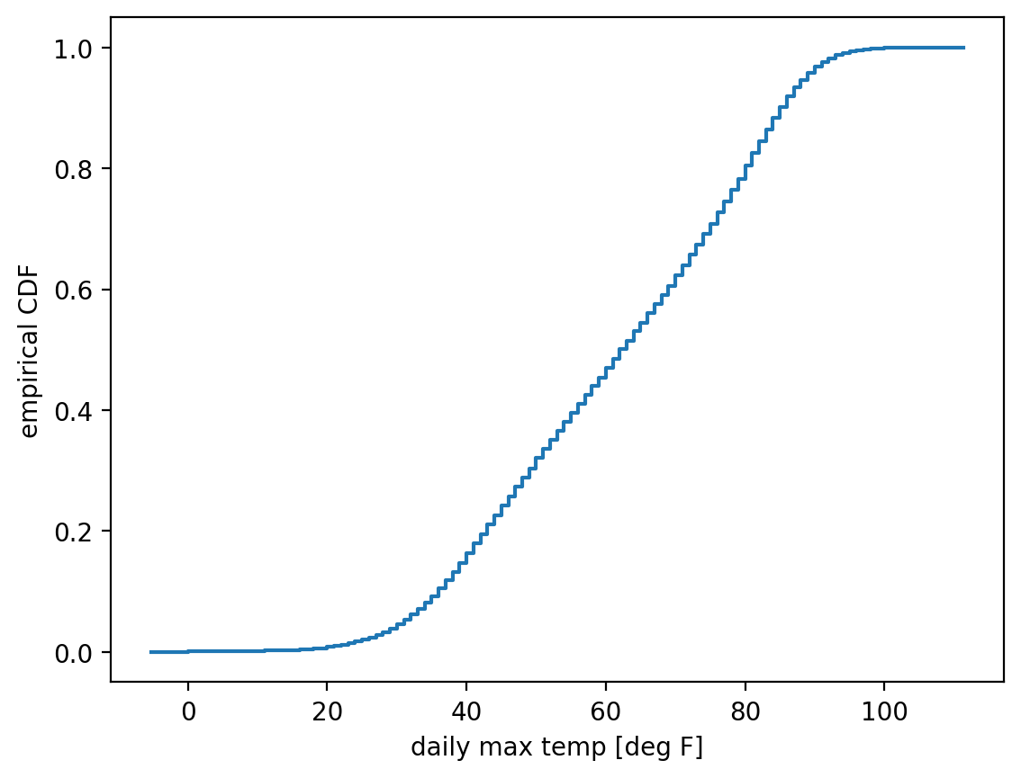
Alright, let’s finally plot that:
fig, ax = plt.subplots()  # create the overall figure and the set of axes we'll plot on.
ecdf_temp_max.cdf.plot(ax=ax)  # plot the CDF onto the `ax` object we just created.
ax.set_xlabel("daily max temp [deg F]")  # label the x axis
ax.set_ylabel("empirical CDF")  # label the y axis
Text(0, 0.5, 'empirical CDF')
Alternative: use ax.plot
Here, again, there are multiple ways of accomplishing the same thing. Above, we used the builtin plot method of the ecdf_temp_max.cdf object. We could instead have used matplotlib functions: ax.plot(ecdf_temp_max.cdf.quantiles, ecdf_temp_max.cdf.probabilities) to get essentially the same thing.
Empirical PDFs#
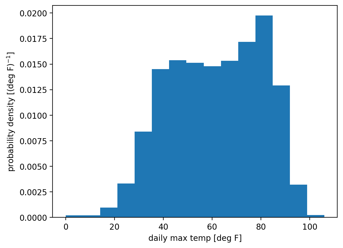
Recall that an empirical probability density function is really just a histogram, crucially with the count in each bin normalized, i.e. divided, by the width of that bin.
We can get this most directly using matplotlib’s hist function and setting density=True:
plt.hist(ds_cp["temp_max"], bins=15, density=True)
plt.xlabel("daily max temp [deg F]")
plt.ylabel(r"probability density [(deg F)$^{-1}$]")
Text(0, 0.5, 'probability density [(deg F)$^{-1}$]')