The τ ≈ 1 sweet spot for emission to space
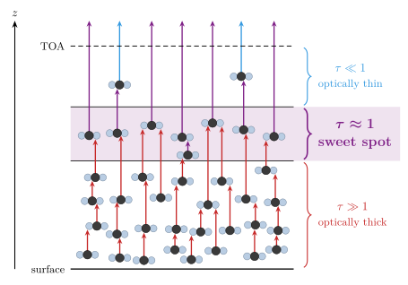
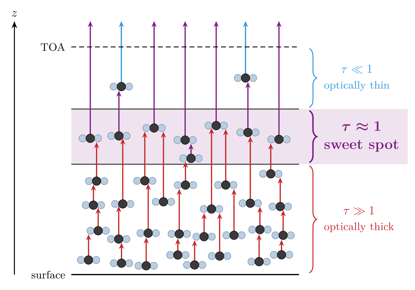
Each CO₂ molecule emits one photon straight up, and the photon is absorbed by the first molecule directly above it. Optical depth τ is measured downward from the top of the atmosphere (TOA), so it is small near the top and large near the surface.
- Optically thin (τ ≪ 1): both photons emitted here escape to space, but there are only two molecules to emit them.
- τ ≈ 1: eight molecules emit, and five of their photons escape.
- Optically thick (τ ≫ 1): 27 molecules emit, and every one of their photons is absorbed before it gets out.
Five of the seven photons that reach space therefore come from the τ ≈ 1 layer. Higher up there are too few emitters, and lower down there is too much absorber overhead. In a real atmosphere, emission to space per unit height likewise peaks near τ ≈ 1.
Each photon’s color shows which layer emitted it: blue for the optically thin layer, purple for the τ ≈ 1 layer and red for the optically thick layers. The colors go from coldest to warmest, since temperature falls with height in the troposphere.
The notes for instructors cover what the cartoon simplifies, the physics behind it and some discussion questions, and give a caption and alt text ready to paste.
Download
- PDF and SVG, both vector graphics
- PNG, 300 dpi
- sweetspot.tex: the TikZ drawing, as a standalone LaTeX document
- make_sweetspot.py: the Python script that places the molecules and writes
sweetspot.tex
Credit
The figure redraws Fig. 3 of Nadir Jeevanjee, “Climate sensitivity from radiative-convective equilibrium: A chalkboard approach,” American Journal of Physics 91, 731–745 (2023), https://doi.org/10.1119/5.0135727, the article’s cartoon of emission to space from layers of increasing optical depth. The article is © 2023 its author and published under the CC BY 4.0 license. My changes: the original’s three panels became a single column, the τ ≈ 1 layer now sends more photons to space than the optically thin layer (in the original each sends three), the molecules are drawn as linear O=C=O, and each photon’s color shows the layer that emitted it.
My own work on the figure is in the public domain under CC0, like the rest of this gallery. If you reuse the figure, please keep the credit to Jeevanjee’s article.
Changing it
The layout, the positions of the optically thin and τ ≈ 1 molecules, and the height and molecule count of each optically thick row are constants near the top of make_sweetspot.py, which needs only Python and NumPy. The optically thick molecules are scattered at random about their rows. An optional argument sets the random seed, which defaults to 5, and some seeds find no valid placement. The script stops with an error, before it writes sweetspot.tex, if a photon would escape or be absorbed other than as intended or if two molecules would overlap. Compile sweetspot.tex with any LaTeX engine, for example pdflatex sweetspot.tex. The design notes give the reasons behind each choice in the drawing.