Answer Key for HW06: hypothesis tests

⚠️⚠️⚠️ TOTAL POINTS POSSIBLE: 26 ⚠️⚠️⚠️¶

Preliminaries¶

Import needed python packages¶

Load the Central Park data¶

Compare the $t$ and normal distributions¶

In class, we learned that for hypothesis testing of differences in means, the test statistic is called Student’s $t$ or just $t$. The $t$ distribution is similar but not identical to the standard normal distribution, especially for small sample sizes. Its exact shape depends on the degrees of freedom, denoted $\nu$. For the difference in two means, this is simply $\nu=N_1+N_2-2$, where $N_1$ and $N_2$ are the sample sizes of the first and second samples, respectively.

Using scipy.stats.t.pdf and scipy.stats.norm.pdf, plot the PDFs of both distributions spanning from -5 to 5. For the $t$ distribution, overlay 3 different versions on the same axes: $\nu=1, 10$, and 100. Add a legend labeling each of these and the normal.

This demonstrates that, as the sample sizes grow, the $t$ distribution increasingly is well approximated by the standard normal. (In fact, it holds mathematically that the $t$ distribution approaches the standard normal exactly as $\nu\rightarrow\infty$.)

⚠️ POINTS: 4¶

One for the normal and one each for the three t distributions.

✅ ANSWER¶

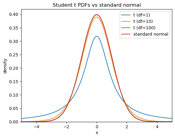
Find the most helpful online resources on $t$ tests you can find¶

There are tons of great resources that are available online and completely free. These include blog posts, YouTube videos, tutorials in the documentation to statistical software packages, whole semester-length university classes that have been pre-recorded, and more. (The course resources page lists just a few.) An important but overlooked skill (you could call it a meta skill) for scientists and engineers is learning to make use of these resources.

For this assignment, search the web to find the best two different resources you can. They can be any of the types listed above or something else.

• For each resource: provide the URL to the resource and describe how you found it.

• If it’s a YouTube video, embed the video in your Jupyter notebook.

• Write summaries in your own words of what each resource conveys.

• Describe one or more things that each resource helped you understand.

• Describe one or more things that each resource did not help you with, either because it was missing or was included but you’re still unclear on it.

• Rank the two resources: which was more helpful and why?

⚠️ POINTS: 10¶

One each, per resource, for the link, summary, description of things it helped you understand, and description of things it didn’t help you with. Two points for the ranking and discussion.

✅ ANSWER¶

There’s no single right answer here...this one was up to you!

Write your own functions for computing the $t$ statistic and $p$ value¶

⚠️ POINTS: 4¶

Two each for each function

✅ ANSWER¶

Compute t tests from CP dataset¶

Specifically, for each of the following pairs of samples from the Central Park dataset:

1. Across all years 1869-2022, monthly average precipitation in September vs. in January.

2. Average annual sum of cooling degree days for the period 1971-2000 vs. 2001-2022.

Use numpy.isclose to explicitly test your values against the results of scipy.stats.ttest_ind.

⚠️ POINTS: 8¶

Four for each pair: one for the data prep, one for computing the t values, one for computing the p values, and one for comparing your functions to scipy.

✅ ANSWER: September vs. January precip¶

✅ ANSWER: 1971-2000 vs. 2001-2022 cooling degree days¶

Extra credit¶

⚠️ EXTRA CREDIT POINTS: For each Q, up to 5% of possible non-extra credit points¶

Decide for yourself what you earned, between 0% and 5%, based on what was asked for.

Compute the $t$ test for two or more salient differences-in-mean for your final project.¶

Find at least two pairs of sample means from your datasets whose difference are scientifically interesting for your project. Perform the $t$ test for each. Report the numerical values of the $t$ statistic, $p$ value, degrees of freedom. Describe your interpretation of the $t$ test from a statistical perspective. Also describe your interpretaiton from a physical/scientific perspective.

✅ ANSWER¶

This will depend on your dataset.

Create a dedicated conda environment for this course¶

The Resources page explains why it’s a good idea to create separate virtual environments for different projects/classes/ etc. using the Anaconda/conda environment manager. For this extra credit opportunity, create a dedicated environment using Anaconda Navigator or the conda command line tool. The environment must be created specifically for this purpose; you could name it eas42000 or eas-a4200 for example.

To show that you have done this, include the following cell in your notebook.

✅ ANSWER¶

Your answer will be the output of the above code. If it shows that the active python and jupyter are inside the directory for the environment you created, and that this environment is what’s active, then you get full credit.